8 December, 2023
Using Machine Learning to Optimize Entries
During the week, I found a superbly helpful 'Machine Learning in Finance' guide on X that used clustering to group price behavior into different groups.
Here is a link to the clustering code by Danny Groves.
Like many educational insights on X (in particular), I typically bookmark to save for later and often forget to check. So, in an effort to change that,
I thought I would set myself the challenge of playing around with Danny's code and seeing a) what I could add and b) how I might tie it to something I have built in the past.
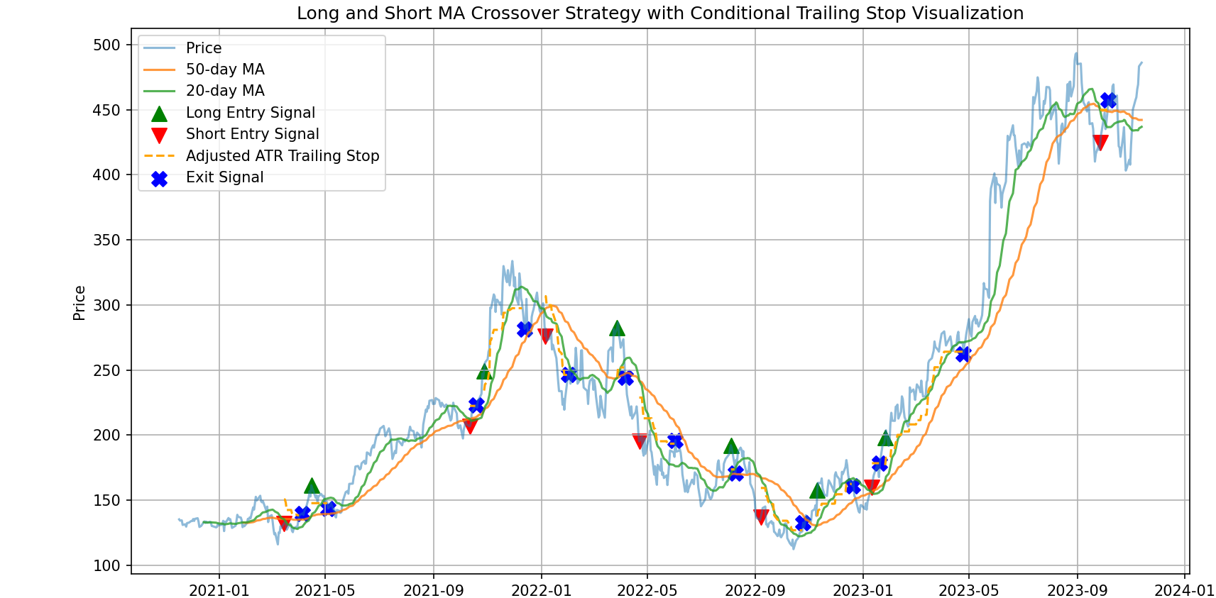
The strategy below takes the MA Crossover with ATR Trailing Stop Strategy and uses ML to increase the proability of successful entries. Basically, I took the cluster approach,
identified the three clusters that ranked best as a function of high returns and low volatility, and only entered trades when the MA crossover was within one of these
three 'good_clusters'. Instead of then trying to predict where price would go post-entry, I kept the regular ATR trailing stop approach that adjusts with increasing price.
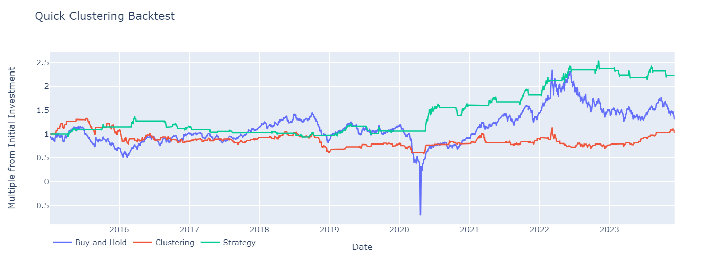
The results (when tested on OIL futures) are quite good: lowest drawdown and highest return. When I tested on other stocks/futures (SPY, GC=F, BTC-USD),
the results aren't as strong. In some cases, the clustering algorithm alone performs better - it all depends on the length of training data, the ATR multiplier chosen and the
Moving Average lengths.
My next post will compare how this model performs in different markets and environments.
(For simplicity sake, this is a long-only strategy and ignores any slippage, commisions etc.)
import pandas as pd
import numpy as np
import matplotlib.pyplot as plt
import yfinance as yf
from sklearn.cluster import KMeans
from kneed import KneeLocator
from sklearn.ensemble import RandomForestClassifier
from sklearn.metrics import accuracy_score, precision_score, confusion_matrix
from sklearn.preprocessing import StandardScaler
import seaborn as sns
import plotly.express as px
from plotly import graph_objects as go

import yfinance as yf
import numpy as np

# Download SPY df
df = yf.download('CL=F').reset_index()

# Distance from the moving averages
for m in [10, 20, 30, 50, 100]:
    df[f'feat_dist_from_ma_{m}'] = df['Close'] / df['Close'].rolling(m).mean() - 1

# Distance from n day max/min
for m in [3, 5, 10, 15, 20, 30, 50, 100]:
    df[f'feat_dist_from_max_{m}'] = df['Close'] / df['High'].rolling(m).max() - 1
    df[f'feat_dist_from_min_{m}'] = df['Close'] / df['Low'].rolling(m).min() - 1

# Price distance
for m in [1, 2, 3, 4, 5, 10, 15, 20, 30, 50, 100]:
    df[f'feat_price_dist_{m}'] = df['Close'] / df['Close'].shift(m) - 1

# Add EMA features
for m in [10, 20, 30, 50, 100]:
    ema = df['Close'].ewm(span=m, adjust=False).mean()
    df[f'feat_dist_from_ema_{m}'] = df['Close'] / ema - 1

# Drop NaN values created by rolling functions
df = df.dropna()

# Split the df into training and testing sets based on date
df_train = df[df['Date'] < '2015-01-01'].reset_index(drop=True)
df_test = df[df['Date'] >= '2015-01-01'].reset_index(drop=True)

print(df_train.columns)
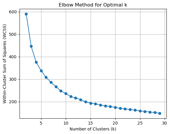
Next, we find the optimal number of clusters to work with. This is important because if we have too many clusters, many will be almost identical. By visually inspecting where WSS curve flattens or by using predict function, we can find optimal number of clusters to work with.
feat_cols = [col for col in df.columns if 'feat' in col]

X_train = df_train[feat_cols]

# List to store the within-cluster sum of squares for different k values
wcss = []
k_range = range(2, 30)

# Calculate WCSS for a range of k values
for k in k_range:
    kmeans = KMeans(n_clusters=k, random_state=42, n_init='auto')
    kmeans.fit(X_train)
    wcss.append(kmeans.inertia_)

# Use KneeLocator to find the elbow point in the WCSS curve
elbow_locator = KneeLocator(k_range, wcss, curve='convex', direction='decreasing')
optimal_k = elbow_locator.elbow

print(f'Optimal k: {optimal_k}')

# Plotting the elbow curve
plt.plot(k_range, wcss, marker='o')
plt.title('Elbow Method for Optimal k')
plt.xlabel('Number of Clusters (k)')
plt.ylabel('Within-Cluster Sum of Squares (WCSS)')
plt.grid(True)
plt.show()

# Create a KMeans instance with the optimal number of clusters
optimal_kmeans = KMeans(n_clusters=optimal_k, random_state=42, n_init='auto')
optimal_kmeans.fit(X_train)

# Predict the clusters for the observations
df_train['cluster'] = optimal_kmeans.predict(X_train)
Optimal k: 9
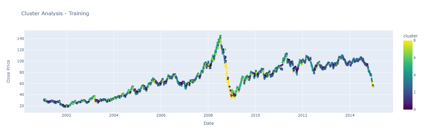
By visualizing the clusters, we can see which ones perform well in strong positive market environments
# Standardize features
scaler = StandardScaler()
df_scaled = scaler.fit_transform(df_train[feat_cols])

# Fit the KMeans model with the number of clusters as seen in the image (6 clusters)
kmeans = KMeans(n_clusters=10, random_state=42)
df_train['cluster'] = kmeans.fit_predict(df_scaled)

# Create a scatter plot using plotly express
fig = px.scatter(df_train, x='Date', y='Close', color='cluster',
                 title="Cluster Analysis - Training",
                 labels={'Close': 'Close Price'}, color_continuous_scale='Viridis')
fig.show()
While visually inspecting clusters, I find it important too to reaffirm what we believe by finding optimal clusters as a function of high returns and low volatility.
# Calculating daily returns
df_train['daily_return'] = df_train['Close'].pct_change()

# Grouping by cluster and calculating the mean daily return for each cluster
mean_cluster_returns = df_train.groupby('cluster')['daily_return'].mean()

# Calculating standard deviation (volatility) for each cluster
cluster_volatility = df_train.groupby('cluster')['daily_return'].std()

# Combining the returns and volatility into a single DataFrame
cluster_performance = pd.DataFrame({
    'return': mean_cluster_returns,
    'volatility': cluster_volatility
})

# Ranking clusters based on high returns and low volatility
# Lower rank is better for volatility, higher rank is better for returns
cluster_performance['return_rank'] = cluster_performance['return'].rank(ascending=False)
cluster_performance['volatility_rank'] = cluster_performance['volatility'].rank(ascending=True)

# Overall score to identify top clusters - lower score is better
cluster_performance['score'] = cluster_performance['return_rank'] + cluster_performance['volatility_rank']

# Selecting top 3 clusters based on the combined score
top_clusters = cluster_performance.nsmallest(3, 'score').index.tolist()

print(f"Top 3 clusters for the strategy: {top_clusters}")
Top 3 clusters for the strategy: [0, 2, 3]
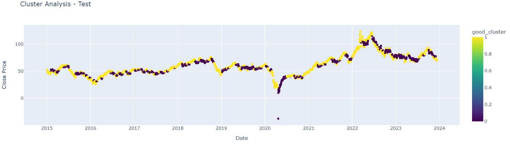
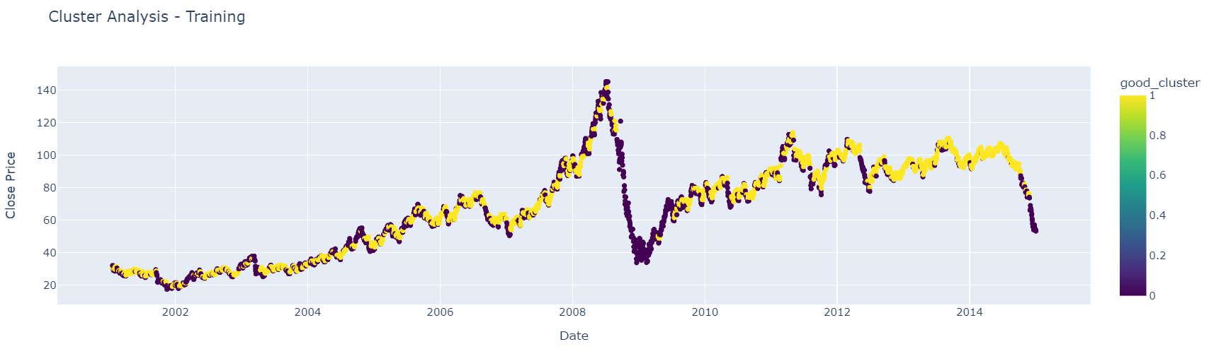
Then, to see if we do have a workable system, good clusters and bad clusters are grouped together into two different groups. First, we see how it looks on training data and then on test data.
# For visualization, classify clusters into 'good' and 'bad' based on the user's input.

good_clusters = [0, 2, 3]
df_scaled = scaler.fit_transform(df_train[feat_cols])
df_train['cluster'] = kmeans.fit_predict(df_scaled)


# Map the clusters to good and bad
df_train['good_cluster'] = df_train['cluster'].apply(lambda x: 1 if x in good_clusters else 0.0)

# Create a scatter plot using plotly express
fig = px.scatter(df_train, x='Date', y='Close', color='good_cluster',
                 title="Cluster Analysis - Test",
                 labels={'Close': 'Close Price'}, color_continuous_scale=px.colors.sequential.Viridis)
fig.show()
# Standardize features
scaler = StandardScaler()
df_scaled = scaler.fit_transform(df_test[feat_cols])

# Fit the KMeans model with the number of clusters as seen in the image (6 clusters)
kmeans = KMeans(n_clusters=9, random_state=42)
df_test['cluster'] = kmeans.fit_predict(df_scaled)

# Create a scatter plot using plotly express
fig = px.scatter(df_test, x='Date', y='Close', color='cluster',
                    title="Cluster Analysis - Test",
                    labels={'Close': 'Close Price'}, color_continuous_scale='Viridis')
fig.show()
The strategy remains almost identical (minus the shorting) as in my previous post with the addition of the 'good_cluster' check within the entry logic.
# Calculating moving averages
df_test['MA50'] = df_test['Close'].rolling(window=50).mean()
df_test['MA20'] = df_test['Close'].rolling(window=10).mean()

df_test['cluster'] = kmeans.fit_predict(df_scaled)
df_test['good_cluster'] = df_test['cluster'].apply(lambda x: 1 if x in good_clusters else 0.0)

# Function to calculate Average True Range (ATR)
def calculate_atr(df_test, period=21):
    df_test['high_low'] = df_test['Close'].diff()
    df_test['high_close'] = np.abs(df_test['Close'] - df_test['Close'].shift())
    df_test['low_close'] = np.abs(df_test['Close'] - df_test['Close'].shift())
    df_test['tr'] = df_test[['high_low', 'high_close', 'low_close']].max(axis=1)
    atr = df_test['tr'].rolling(window=period).mean()
    return atr

# Calculating ATR
df_test['ATR'] = calculate_atr(df_test)

# Setting the ATR multiplier
atr_multiplier = 3

# Identifying entry points for both long and short positions
df_test['Entry_Signal_Long'] = np.where((df_test['MA20'] > df_test['MA50']) & (df_test['MA20'].shift(1) <= df_test['MA50'].shift(1)), 1, 0)
df_test['Entry_Signal_Short'] = np.where((df_test['MA20'] < df_test['MA50']) & (df_test['MA20'].shift(1) >= df_test['MA50'].shift(1)), 1, 0)

# Initialize columns for position and trailing stop
df_test['In_Position'] = 0
df_test['Adjusted_Trailing_Stop'] = np.nan

# Variables to track position, trailing stop, and exit points
in_position = False
trailing_stop = 0
position_type = None
exit_points = []
trades = []
current_trade = {'Entry': None, 'Exit': None}

# Looping through the df_test to adjust position, trailing stop logic, and identify exit points
for index, row in df_test.iterrows():
    if row['Entry_Signal_Long'] == 1 and not in_position and row['good_cluster'] == 1:
        trailing_stop = row['Close'] - (row['ATR'] * atr_multiplier)
        current_trade['Entry'] = (index, row['Close'])
        in_position = True
        position_type = 'long'

    if in_position:
        if position_type == 'long':
            current_trailing_stop = row['Close'] - (row['ATR'] * atr_multiplier)
            trailing_stop = max(trailing_stop, current_trailing_stop)

        # Exit conditions
        if (position_type == 'long' and row['Close'] < trailing_stop):#  or (position_type == 'short' and row['Close'] > trailing_stop):
            in_position = False
            exit_points.append(index)
            current_trade['Exit'] = (index, row['Close'])
            trades.append(current_trade)
            current_trade = {'Entry': None, 'Exit': None}
            df_test.at[index, 'Adjusted_Trailing_Stop'] = np.nan
        else:
            df_test.at[index, 'Adjusted_Trailing_Stop'] = trailing_stop
    else:
        df_test.at[index, 'Adjusted_Trailing_Stop'] = np.nan

    df_test.at[index, 'In_Position'] = int(in_position)

# Applying fillna() to ensure trailing stop is only plotted when in a position
df_test['Plot_Trailing_Stop'] = df_test['Adjusted_Trailing_Stop'].where(df_test['In_Position'] == 1)
from plotly import graph_objects as go
import numpy as np
df_test['pct_change'] = df_test['Close'].pct_change()
df_test['signal'] = df_test['good_cluster'].shift(1)
df_test['equity_cluster'] = np.cumprod(1+df_test['signal']*df_test['pct_change'])
df_test['equity_buy_and_hold'] = np.cumprod(1+df_test['pct_change'])
# Calculate the cumulative product of equity for the strategy
df_test['In_Position'] = df_test['In_Position'].shift(1)
df_test['equity_strategy'] = np.cumprod(1 + df_test['In_Position'] * df_test['pct_change'])
fig = go.Figure()
fig.add_trace(
go.Line(x=df_test['Date'], y=df_test['equity_buy_and_hold'], name='Buy and Hold')
)
fig.add_trace(
go.Line(x=df_test['Date'], y=df_test['equity_cluster'], name='Clustering')
)
fig.add_trace(
go.Line(x=df_test['Date'], y=df_test['equity_strategy'], name='Strategy')
)
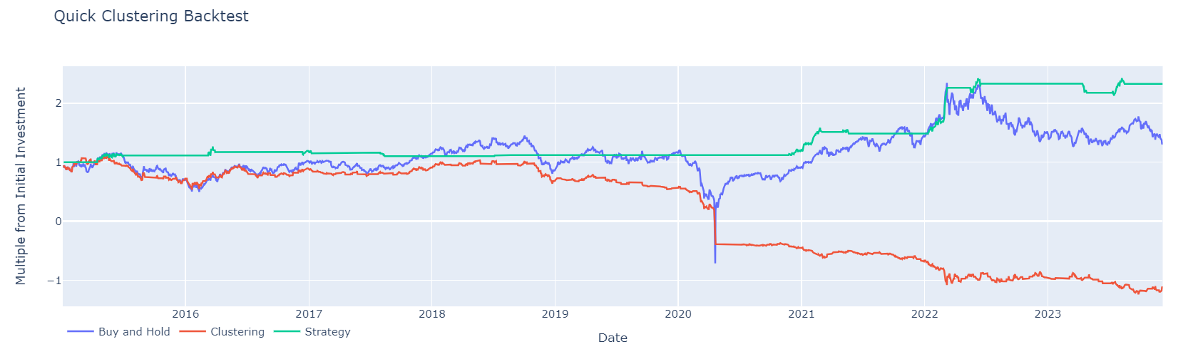
fig.update_layout(
title_text='Quick Clustering Backtest',
legend={'x': 0, 'y':-0.05, 'orientation': 'h'},
xaxis={'title': 'Date'},
yaxis={'title': 'Multiple from Initial Investment'}
)
def get_max_drawdown(col):
drawdown = col / col.cummax() - 1
return 100 * drawdown.min()

def calculate_cagr(col, n_years):
    cagr = (col.values[-1] / col.values[0]) ** (1 / n_years) - 1
    return 100 * cagr

print('Maximum Drawdown Buy and Hold:', get_max_drawdown(df_test['equity_buy_and_hold']))
print('Maximum Drawdown Clustering:', get_max_drawdown(df_test['equity_cluster']))
print('Maximum Drawdown Strategy:', get_max_drawdown(df_test['equity_strategy']))

print('')

n_years = (df_test['Date'].max() - df_test['Date'].min()).days / 365.25

print('CAGR Buy and Hold:', calculate_cagr(df_test['equity_buy_and_hold'].dropna(), n_years))
print('CAGR Clustering:', calculate_cagr(df_test['equity_cluster'].dropna(), n_years))
print('CAGR Random Strategy:', calculate_cagr(df_test['equity_strategy'].dropna(), n_years))
Maximum Drawdown Buy and Hold: -149.24747973382892
Maximum Drawdown Clustering: -55.67676221505267
Maximum Drawdown Strategy: -32.73684867226392
CAGR Buy and Hold: 4.037706652182704
CAGR Clustering: 0.6633401650248505
CAGR Random Strategy: 9.41790316427702